Link Functions in clmstan

Overview

clmstan supports 11 link functions for cumulative link models—more than any other CLM package. This article explains: - The mathematical properties of each link function - Visual comparison of their CDFs - How to choose the best link for your data

library(clmstan)
library(ordinal)
library(loo)
data(wine)

Link Functions at a Glance

Standard Links (5)

Standard links have no adjustable parameters:

Link	Distribution	Characteristics
logit	Logistic	Default, proportional odds interpretation
probit	Normal	Symmetric, latent variable interpretation
cloglog	Gumbel (max)	Right-skewed, proportional hazards
loglog	Gumbel (min)	Left-skewed
cauchit	Cauchy	Heavy tails, robust to outliers

Flexible Links (6)

Flexible links have parameters that can be fixed or estimated from data:

Link	Parameters	Special Cases
tlink	$\text{df} > 0$	$\text{df} \to \infty$ : probit
aranda_ordaz	$\lambda > 0$	$\lambda = 1$ : logit; $\lambda \to 0$ : cloglog
gev	$\xi \in \mathbb{R}$	$\xi = 0$ : loglog (Gumbel)
sp	$r > 0$ , base	$r = 1$ : base distribution
log_gamma	$\lambda \in \mathbb{R}$	$\lambda = 0$ : probit
aep	$\theta_1, \theta_2 > 0$	$\theta_1 = \theta_2 = 2$ : similar to probit

supported_links()
#>  [1] "logit"        "probit"       "cloglog"      "loglog"       "cauchit"     
#>  [6] "tlink"        "aranda_ordaz" "gev"          "sp"           "log_gamma"   
#> [11] "aep"

Visual Comparison

The cumulative distribution function (CDF) determines how probabilities are mapped to the latent scale. Different CDFs produce different model behavior, especially for extreme categories.

Standard Link CDFs

x <- seq(-4, 4, length.out = 200)

cdfs <- data.frame(
  x = x,
  logit = plogis(x),
  probit = pnorm(x),
  cloglog = 1 - exp(-exp(x)),
  loglog = exp(-exp(-x)),
  cauchit = pcauchy(x)
)

par(mar = c(4, 4, 2, 1))
plot(x, cdfs$logit, type = "l", lwd = 2, col = 1,
     xlab = "x", ylab = "F(x)", main = "Standard Link CDFs",
     ylim = c(0, 1))
lines(x, cdfs$probit, lwd = 2, col = 2)
lines(x, cdfs$cloglog, lwd = 2, col = 3)
lines(x, cdfs$loglog, lwd = 2, col = 4)
lines(x, cdfs$cauchit, lwd = 2, col = 5, lty = 2)
legend("bottomright",
       legend = c("logit", "probit", "cloglog", "loglog", "cauchit"),
       col = 1:5, lwd = 2, lty = c(1, 1, 1, 1, 2))
abline(h = 0.5, lty = 3, col = "gray")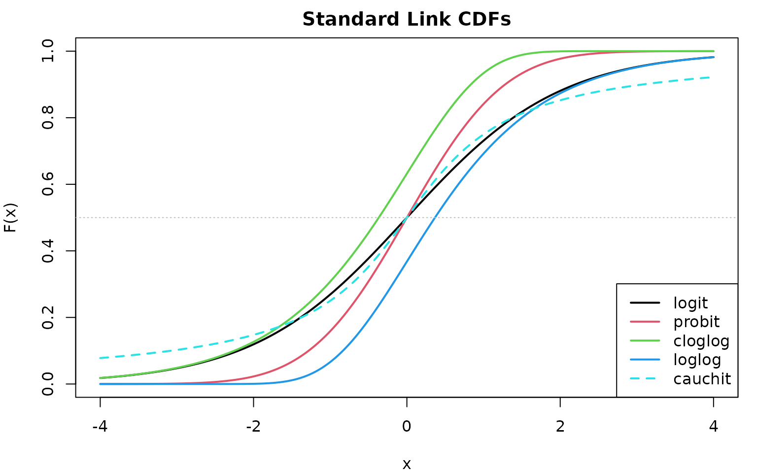

Key observations:

logit and probit: Nearly identical symmetric curves
cloglog: Right-skewed (slower approach to 1)
loglog: Left-skewed (slower approach to 0)
cauchit: Heavy tails (slower approach to both 0 and 1)

t-link: Adjustable Tail Weight

The t-link interpolates between cauchit ( $\text{df}=1$ ) and probit ( $\text{df} \to \infty$ ):

x <- seq(-4, 4, length.out = 200)

par(mar = c(4, 4, 2, 1))
plot(x, pnorm(x), type = "l", lwd = 2, col = "black", lty = 2,
     xlab = "x", ylab = "F(x)", main = "t-link CDFs (varying df)",
     ylim = c(0, 1))
lines(x, pt(x, df = 1), lwd = 2, col = 2)
lines(x, pt(x, df = 2), lwd = 2, col = 3)
lines(x, pt(x, df = 3), lwd = 2, col = 4)
lines(x, pt(x, df = 4), lwd = 2, col = 5)
lines(x, pt(x, df = 8), lwd = 2, col = 6)
lines(x, pt(x, df = 30), lwd = 2, col = 7)
legend("bottomright",
       legend = c("probit (df=Inf)", "df=1 (Cauchy)", "df=2", "df=3",
                  "df=4", "df=8", "df=30"),
       col = c(1, 2:7), lwd = 2, lty = c(2, rep(1, 6)))
abline(h = 0.5, lty = 3, col = "gray")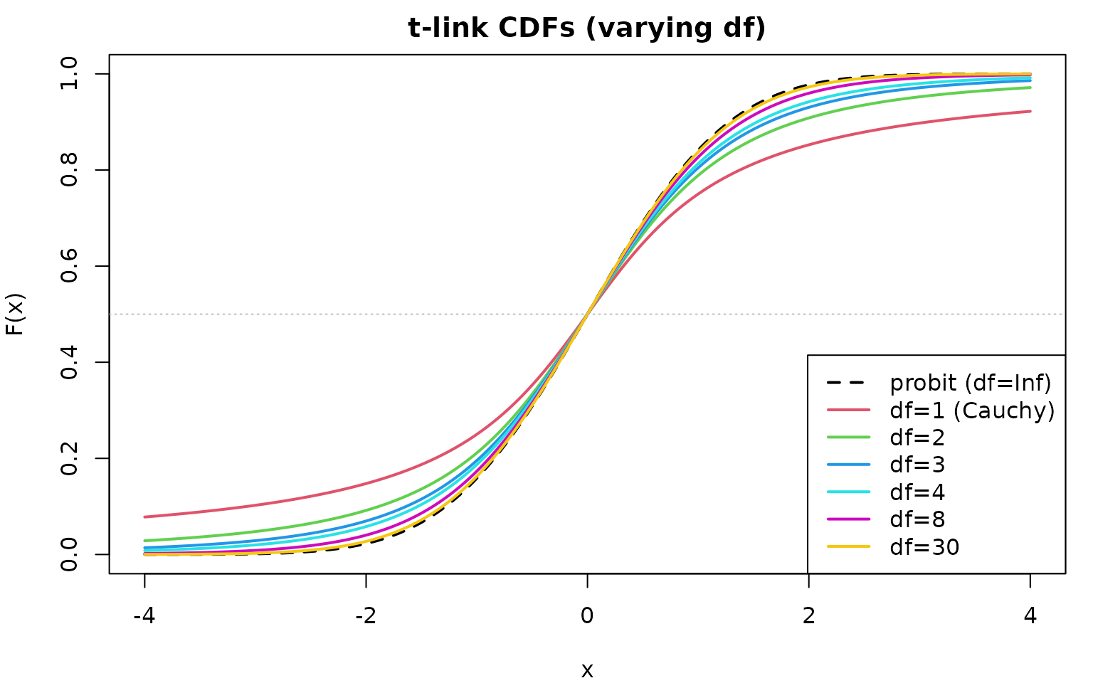

Guidelines for df:

df	Tail behavior	Equivalent to
1	Very heavy	cauchit
2–3	Heavy	—
4–8	Moderate	—
$>30$	Light	probit

Practical Comparison

Fitting Models with Different Links

We compare link functions using the wine dataset. First, we fit models with the five standard links:

set.seed(42)

fit_logit <- clm_stan(rating ~ temp + contact, data = wine, link = "logit",
                      chains = 2, iter = 1000, warmup = 500, refresh = 0)

fit_probit <- clm_stan(rating ~ temp + contact, data = wine, link = "probit",
                       chains = 2, iter = 1000, warmup = 500, refresh = 0)

fit_cloglog <- clm_stan(rating ~ temp + contact, data = wine, link = "cloglog",
                        chains = 2, iter = 1000, warmup = 500, refresh = 0)

fit_loglog <- clm_stan(rating ~ temp + contact, data = wine, link = "loglog",
                       chains = 2, iter = 1000, warmup = 500, refresh = 0)

fit_cauchit <- clm_stan(rating ~ temp + contact, data = wine, link = "cauchit",
                        chains = 2, iter = 1000, warmup = 500, refresh = 0)

Next, we fit models with the six flexible links. These links have parameters that are estimated from the data:

fit_tlink <- clm_stan(rating ~ temp + contact, data = wine, link = "tlink",
                      link_param = list(df = "estimate"),
                      chains = 2, iter = 1000, warmup = 500, refresh = 0)

fit_aranda <- clm_stan(rating ~ temp + contact, data = wine, link = "aranda_ordaz",
                       link_param = list(lambda = "estimate"),
                       chains = 2, iter = 1000, warmup = 500, refresh = 0)

fit_gev <- clm_stan(rating ~ temp + contact, data = wine, link = "gev",
                    link_param = list(xi = "estimate"),
                    chains = 2, iter = 1000, warmup = 500, refresh = 0)

fit_sp <- clm_stan(rating ~ temp + contact, data = wine, link = "sp",
                   base = "logit", link_param = list(r = "estimate"),
                   chains = 2, iter = 1000, warmup = 500, refresh = 0)

fit_loggamma <- clm_stan(rating ~ temp + contact, data = wine, link = "log_gamma",
                         link_param = list(lambda = "estimate"),
                         chains = 2, iter = 1000, warmup = 500, refresh = 0)

fit_aep <- clm_stan(rating ~ temp + contact, data = wine, link = "aep",
                    link_param = list(theta1 = "estimate", theta2 = "estimate"),
                    chains = 2, iter = 1000, warmup = 500, refresh = 0)

Model Comparison with LOO-CV

We use leave-one-out cross-validation (LOO-CV) to compare predictive performance across all 11 models:

# Compute LOO for standard links
loo_logit <- loo(fit_logit)
loo_probit <- loo(fit_probit)
loo_cloglog <- loo(fit_cloglog)
loo_loglog <- loo(fit_loglog)
loo_cauchit <- loo(fit_cauchit)

# Compute LOO for flexible links
loo_tlink <- loo(fit_tlink)
loo_aranda <- loo(fit_aranda)
loo_gev <- loo(fit_gev)
loo_sp <- loo(fit_sp)
loo_loggamma <- loo(fit_loggamma)
loo_aep <- loo(fit_aep)

# Compare all 11 link functions (sorted by expected log predictive density)
loo_list <- list(
  logit = loo_logit,
  probit = loo_probit,
  cloglog = loo_cloglog,
  loglog = loo_loglog,
  cauchit = loo_cauchit,
  tlink = loo_tlink,
  aranda_ordaz = loo_aranda,
  gev = loo_gev,
  sp = loo_sp,
  log_gamma = loo_loggamma,
  aep = loo_aep
)
loo::loo_compare(loo_list)
#>              elpd_diff se_diff
#> probit        0.0       0.0   
#> tlink        -0.5       0.4   
#> logit        -0.6       0.5   
#> gev          -0.9       0.4   
#> cloglog      -1.0       1.6   
#> sp           -1.3       0.6   
#> aranda_ordaz -1.3       0.5   
#> loglog       -2.3       1.8   
#> log_gamma    -4.8       1.0   
#> aep          -5.6       1.7   
#> cauchit      -7.6       2.7

How to interpret:

Models are sorted by expected log predictive density (best first)
elpd_diff: Difference from the best model (0 = best)
se_diff: Standard error of the difference
Rule of thumb: If $|\texttt{elpd\_diff}| < 2 \times \texttt{se\_diff}$ , the difference is not significant

Note: WAIC (Widely Applicable Information Criterion) is also available via waic(fit). LOO-CV is generally preferred as it provides diagnostics for problematic observations (Pareto k values).

Interpreting Results

Coefficient comparison across standard links:

coefs <- data.frame(
  logit = coef(fit_logit),
  probit = coef(fit_probit),
  cloglog = coef(fit_cloglog),
  loglog = coef(fit_loglog),
  cauchit = coef(fit_cauchit)
)
round(coefs, 3)
#>            logit probit cloglog loglog cauchit
#> 1|2        0.000  0.000   0.000  0.000   0.000
#> 2|3        2.678  1.559   2.185  1.520   5.042
#> 3|4        4.918  2.888   3.656  2.977   7.330
#> 4|5        6.527  3.824   4.557  4.259   9.660
#> tempwarm   2.458  1.521   1.631  1.551   2.126
#> contactyes 1.501  0.877   0.879  0.899   1.310

Note: Coefficients are on different scales depending on the link function. Direct comparison of magnitudes is not meaningful; compare signs and relative importance instead.

Estimated link parameters for flexible links:

# Combine all flexible link parameter estimates into one table
link_params_all <- rbind(
  cbind(link = "tlink", summary(fit_tlink)$link_params),
  cbind(link = "aranda_ordaz", summary(fit_aranda)$link_params),
  cbind(link = "gev", summary(fit_gev)$link_params),
  cbind(link = "sp", summary(fit_sp)$link_params),
  cbind(link = "log_gamma", summary(fit_loggamma)$link_params),
  cbind(link = "aep", summary(fit_aep)$link_params)
)
link_params_all
#>           link variable       mean         sd       2.5%         50%      97.5%
#> 1        tlink       df 19.9512987 15.1321539  2.9847032 15.71479200 59.2091042
#> 2 aranda_ordaz   lambda  1.1162084  1.0284254  0.2799335  0.81190743  4.0844419
#> 3          gev       xi -0.2751134  0.1721647 -0.6038121 -0.27820272  0.0847995
#> 4           sp        r  1.0396368  0.3859994  0.4388587  0.98611015  2.0196172
#> 5    log_gamma   lambda -0.1094952  0.6567701 -1.5554499 -0.02322702  1.0280382
#> 6          aep   theta1  0.9577882  0.7939766  0.2796018  0.68772842  3.1507534
#> 7          aep   theta2  1.1513928  0.8045819  0.3285152  0.91051747  3.4711979
#>        rhat   ess_bulk  ess_tail
#> 1 0.9999437 670.638466 583.95919
#> 2 1.0098237 239.821331 271.24284
#> 3 1.0017794 390.305936 363.24424
#> 4 1.0018915 250.191143 322.13696
#> 5 1.8545622   2.979474 109.62488
#> 6 1.0690526  30.480243  63.40078
#> 7 1.0551250  39.044523 241.81909

Quick Reference

Link	Usage	When to use
logit	`link = "logit"`	Proportional odds model
probit	`link = "probit"`	Latent normal variable
cloglog	`link = "cloglog"`	Right-skewed; proportional hazards
loglog	`link = "loglog"`	Left-skewed; mirror of cloglog
cauchit	`link = "cauchit"`	Heavy-tailed errors
tlink	`link = "tlink", link_param = list(df = "estimate")`	Adjustable tail weight
aranda_ordaz	`link = "aranda_ordaz", link_param = list(lambda = "estimate")`	Logit-cloglog interpolation; $\lambda = 1$ is logit
gev	`link = "gev", link_param = list(xi = "estimate")`	Unconstrained skewness; $\xi = 0$ gives loglog
sp	`link = "sp", base = "logit", link_param = list(r = "estimate")`	Adjustable skewness
log_gamma	`link = "log_gamma", link_param = list(lambda = "estimate")`	Generalized probit; $\lambda = 0$ is probit
aep	`link = "aep", link_param = list(theta1 = "estimate", theta2 = "estimate")`	Independent tail shapes

References

Agresti, A. (2010). Analysis of Ordinal Categorical Data (2nd ed.). Wiley.
Albert, J.H., & Chib, S. (1993). Bayesian analysis of binary and polychotomous response data. Journal of the American Statistical Association, 88(422), 669–679.
Aranda-Ordaz, F.J. (1981). On two families of transformations to additivity for binary response data. Biometrika, 68(2), 357–363.
Jiang, X., & Dey, D.K. (2015). Symmetric power link with ordinal response model. In Current Trends in Bayesian Methodology with Applications. CRC Press.
Naranjo, L., Pérez, C.J., & Martín, J. (2015). Bayesian analysis of some models that use the asymmetric exponential power distribution. Statistics and Computing, 25(3), 497–514.
Prentice, R.L. (1976). A generalization of the probit and logit methods for dose response curves. Biometrics, 32(4), 761–768.
Wang, X., & Dey, D.K. (2011). Generalized extreme value regression for ordinal response data. Environmental and Ecological Statistics, 18(4), 619–634.