Introduction to the mhn Package

The mhn package provides density, distribution, quantile, and random generation functions for the Modified Half-Normal (MHN) distribution, plus helpers for its moments and mode. This vignette walks through the basic usage of every exported function.

library(mhn)

The MHN distribution

The MHN( $\alpha$ , $\beta$ , $\gamma$ ) distribution has support on $(0, \infty)$ and density

$f(x \mid \alpha, \beta, \gamma) = \frac{2 \beta^{\alpha/2} \, x^{\alpha-1} \, \exp(-\beta x^2 + \gamma x)} {\Psi[\alpha/2,\, \gamma/\sqrt{\beta}]}, \qquad x > 0,$

where $\alpha > 0$ , $\beta > 0$ , $\gamma \in \mathbb{R}$ , and $\Psi[a, z]$ is the Fox–Wright ${}_1\Psi_1$ function used as the normalising constant (Sun, Kong & Pal 2023). The three parameters control the polynomial factor $x^{\alpha-1}$ , the Gaussian tail $\exp(-\beta x^2)$ , and the exponential tilt $\exp(\gamma x)$ respectively.

Density: `dmhn()`

dmhn() evaluates the density (or log-density) at one or more points:

dmhn(c(0.5, 1, 2), alpha = 2, beta = 1, gamma = 1)
#> [1] 0.4702986 0.7325378 0.1982764
dmhn(1, alpha = 2, beta = 1, gamma = 1, log = TRUE)
#> [1] -0.3112403

It is vectorised over both x and the parameters, with standard R recycling:

dmhn(c(0.5, 1, 1.5), alpha = c(1, 2), beta = 1, gamma = c(0, 1, -1))
#> [1] 0.87878258 0.73253783 0.04310111

x <- c(seq(0.001, 0.3, length.out = 60), seq(0.3, 5, length.out = 140))
plot(x, dmhn(x, alpha = 2, beta = 1, gamma = 1),
     type = "l", lwd = 2, ylab = "density", ylim = c(0, 1),
     main = expression("MHN(" * alpha * ", " * beta * ", " * gamma * ")"))
lines(x, dmhn(x, alpha = 0.5, beta = 1, gamma = 1), lwd = 2, col = "tomato")
lines(x, dmhn(x, alpha = 0.3, beta = 1, gamma = 4), lwd = 2, col = "steelblue")
legend("topright", bty = "n",
       legend = c("(2, 1, 1)    log-concave, mode near 1",
                  "(0.5, 1, 1)  monotone decreasing",
                  "(0.3, 1, 4)  boundary spike + interior bump"),
       col = c("black", "tomato", "steelblue"), lwd = 2)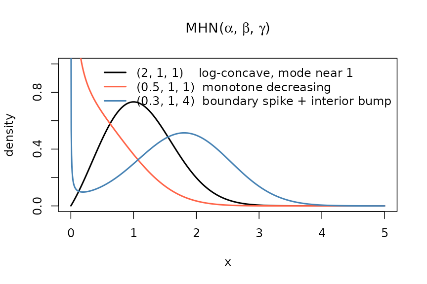

MHN densities for three parameter triples; the steelblue curve sits in the alpha < 1, gamma >> 0 regime where the density combines a boundary divergence at x to 0+ with an interior local maximum near x = 1.8 (Sun et al. 2023, Lemma 3c). The y-axis is clipped at 1; the divergent left tails of the tomato and steelblue curves continue upward beyond the plot.

Distribution function: `pmhn()`

pmhn() returns $P(X \le q)$ (or its complement / log-probability via lower.tail / log.p). For the general case it evaluates the Sun et al. (2023) Lemma 1b series in log space, truncated at the constructive bound $K = \max\{K_1, K_2\}$ from Sun et al. (2023, Supplementary Lemma 10(d)). When the underlying double-precision cancellation in the alternating-sign accumulator for $\gamma < 0$ would exceed the user’s tolerance, the routine falls back to a peak-normalised Boost.Math quadrature (Gauss–Kronrod for $\alpha \ge 1$ , tanh–sinh for $\alpha < 1$ ) of the unnormalised density.

pmhn(c(0.5, 1, 1.5, 2), alpha = 2, beta = 1, gamma = 1)
#> [1] 0.1129101 0.4338796 0.7614259 0.9363038
pmhn(2, alpha = 2, beta = 1, gamma = 1, lower.tail = FALSE)
#> [1] 0.06369619
pmhn(2, alpha = 2, beta = 1, gamma = 1, log.p = TRUE)
#> [1] -0.06581527

A direct cross-check against integrate(dmhn, 0, q) confirms accuracy:

q <- 1.5
ref <- integrate(function(x) dmhn(x, 2, 1, 1), 0, q,
                 rel.tol = 1e-10)$value
all.equal(pmhn(q, 2, 1, 1), ref)
#> [1] TRUE

plot(x, dmhn(x, 2, 1, 1), type = "l", lwd = 2, ylab = "f(x)", main = "Density")
plot(x, pmhn(x, 2, 1, 1), type = "l", lwd = 2, ylab = "F(x)", main = "CDF",
     ylim = c(0, 1))

Density and matching CDF for MHN(2, 1, 1).

Quantile function: `qmhn()`

qmhn() inverts the CDF using a TOMS 748 root-finder bracketed by $[\sqrt{\epsilon}, E(X) + 8 \sqrt{\mathrm{Var}(X)}]$ , expanded as required.

qmhn(c(0.1, 0.5, 0.9), alpha = 2, beta = 1, gamma = 1)
#> [1] 0.4717434 1.0906276 1.8480472

The round-trip identity holds within the inverter’s tolerance:

p <- c(0.01, 0.1, 0.5, 0.9, 0.99)
all.equal(pmhn(qmhn(p, 2, 1, 1), 2, 1, 1), p, tolerance = 1e-6)
#> [1] TRUE

lower.tail and log.p follow the same conventions as qnorm/qgamma:

qmhn(0.95, 2, 1, 1, lower.tail = FALSE)        # = qmhn(0.05)
#> [1] 0.3394014
qmhn(log(0.05), 2, 1, 1, log.p = TRUE)         # same value, log-input
#> [1] 0.3394014

Random generation: `rmhn()`

rmhn(n, alpha, beta, gamma) draws n variates. The default method = "auto" chooses between the special-case shortcuts (sqrt-Gamma for $\gamma = 0$ ; truncated normal for $\alpha = 1$ ), Sun et al. (2023) Algorithms 1 / 3, and the Gao & Wang (2025) Relaxed Transformed Density Rejection (RTDR) sampler. The user can force a single sampler via method = "rtdr" or method = "sun".

rmhn(5, alpha = 2, beta = 1, gamma = 1)
#> [1] 0.3705190 1.1166586 0.9019525 1.3946419 1.1552967

# Vector parameters are recycled to length n.
rmhn(5, alpha = c(1, 2, 3, 4, 5))
#> [1] 0.2046802 0.5574992 0.9775332 0.7787843 1.8248242

set.seed(42)
draws <- rmhn(10000, alpha = 2, beta = 1, gamma = 1)
hist(draws, breaks = 60, probability = TRUE, col = "grey90", border = "white",
     xlab = "x", main = "rmhn(10000, 2, 1, 1)")
lines(x, dmhn(x, 2, 1, 1), lwd = 2, col = "tomato")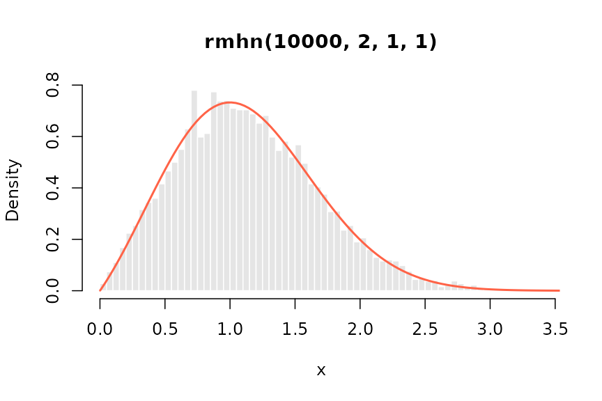

10,000 draws from MHN(2, 1, 1) with the true density overlaid.

Switching method is useful for benchmarking; for the same seed both forced paths produce statistically equivalent samples:

set.seed(1); s_rtdr <- rmhn(5000, 2, 1, 1, method = "rtdr")
set.seed(1); s_sun  <- rmhn(5000, 2, 1, 1, method = "sun")
ks.test(s_rtdr, s_sun)$p.value
#> [1] 0.3274975

Moments and mode

The package provides closed-form / recurrence-based helpers for the common summary statistics (all from Sun et al. 2023, Lemmas 2 and 3):

data.frame(
  Quantity = c("mean", "variance", "skewness", "excess kurtosis", "mode"),
  Function = c("mhn_mean", "mhn_var", "mhn_skewness",
               "mhn_kurtosis", "mhn_mode"),
  Value = c(
    mhn_mean(2, 1, 1),
    mhn_var(2, 1, 1),
    mhn_skewness(2, 1, 1),
    mhn_kurtosis(2, 1, 1),
    mhn_mode(2, 1, 1)
  )
)
#>          Quantity     Function       Value
#> 1            mean     mhn_mean 1.133731086
#> 2        variance      mhn_var 0.281519367
#> 3        skewness mhn_skewness 0.463887428
#> 4 excess kurtosis mhn_kurtosis 0.006868473
#> 5            mode     mhn_mode 1.000000000

When no interior mode exists (e.g. $\alpha < 1$ with $\gamma \le 0$ ), mhn_mode() returns NA:

mhn_mode(0.5, 1, -1)
#> [1] NA

Special cases

The MHN family contains several familiar distributions:

Constraint	Reduction
$\gamma = 0$	$X^2 \sim \mathrm{Gamma}(\alpha/2, \beta)$ (sqrt-Gamma)
$\alpha = 1$	Truncated normal on $(0, \infty)$
$\alpha = 1, \gamma = 0$	Half-normal $\|Z\|, Z \sim N(0, 1/(2\beta))$

The package detects each case (within sqrt(.Machine$double.eps)) and dispatches to the corresponding closed-form R primitive, so dmhn / pmhn / qmhn / rmhn are exact in those regimes:

# gamma = 0: dmhn matches the change-of-variable sqrt-Gamma density.
xx <- c(0.5, 1, 1.5, 2)
mhn_d  <- dmhn(xx, alpha = 2, beta = 1, gamma = 0)
ref_d  <- dgamma(xx^2, shape = 1, rate = 1) * 2 * xx
all.equal(mhn_d, ref_d)
#> [1] TRUE

mu_tn    <- 1 / (2 * 1)
sigma_tn <- 1 / sqrt(2 * 1)
tn_dens  <- function(x) {
  dnorm(x, mu_tn, sigma_tn) / pnorm(0, mu_tn, sigma_tn, lower.tail = FALSE)
}
plot(x, dmhn(x, 1, 1, 1), type = "l", lwd = 2, ylab = "density",
     main = "alpha = 1: MHN reduces to truncated normal")
points(x, tn_dens(x), pch = ".", col = "tomato", cex = 2)
legend("topright", bty = "n",
       legend = c("dmhn(x, 1, 1, 1)", "TN reference"),
       col = c("black", "tomato"), lwd = c(2, NA), pch = c(NA, 19))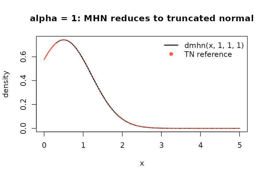

MHN(1, 1, 1) and the equivalent truncated normal density.

References

Sun, J., Kong, M., & Pal, S. (2023). The Modified-Half-Normal distribution: Properties and an efficient sampling scheme. Communications in Statistics – Theory and Methods, 52(5), 1507–1536.

Gao, F. & Wang, H.-B. (2025). Generating modified-half-normal random variates by a relaxed transformed density rejection method. Communications in Statistics – Simulation and Computation.

Robert, C. P. (1995). Simulation of truncated normal variables. Statistics and Computing, 5(2), 121–125.

The MHN distribution

Density: dmhn()

Distribution function: pmhn()

Quantile function: qmhn()

Random generation: rmhn()