Theoretical background of the mhn package

Scope

This vignette is the theoretical companion to Introduction to the mhn Package. The Introduction shows what the four exported functions (dmhn / pmhn / qmhn / rmhn) and their moment helpers do; this note develops the mathematical and algorithmic theory the package implements. We summarise the Modified Half-Normal (MHN) family, the Fox–Wright $\Psi$ function that appears in its normalising constant, and the two sampling schemes the package draws on — Sun, Kong & Pal (2023) and Gao & Wang (2025).

We deliberately keep the treatment compact. Full proofs and the finer numerical considerations live in the original papers (see References). Two implementation-relevant points — the typesetting errata in Sun et al. (2023) that the package silently corrects, and the benchmark-driven rationale for the rmhn(method = "auto") crossover at 25 — are inserted in §4 and §7 where they are most relevant.

The MHN($\alpha$, $\beta$, $\gamma$) family

The MHN distribution has support $(0, \infty)$ and density

$$f(x \mid \alpha, \beta, \gamma) = \frac{2 \beta^{\alpha/2} \, x^{\alpha-1} \, \exp(-\beta x^2 + \gamma x)} {\Psi[\alpha/2,\, \gamma/\sqrt{\beta}]}, \qquad x > 0,$$

with $\alpha > 0$, $\beta > 0$, $\gamma \in \mathbb{R}$. The three parameters control three independent factors of the density kernel:

Parameter	Factor it controls	Role
$\alpha$	$x^{\alpha-1}$	shape
$\beta$	$\exp(-\beta x^2)$	Gaussian tail
$\gamma$	$\exp(\gamma x)$	exponential tilt

Three familiar distributions sit inside the family as exact special cases (Sun et al. 2023, Lemma 6):

Constraint	Reduction
$\gamma = 0$	$X^2 \sim \mathrm{Gamma}(\alpha/2,\, \beta)$, i.e. sqrt-Gamma
$\alpha = 1$	Truncated normal $\mathrm{TN}(\gamma/(2\beta),\, 1/\sqrt{2\beta},\, 0,\, \infty)$
$\alpha = 1,\, \gamma = 0$	Half-normal $\lvert Z \rvert$ with $Z \sim N(0,\, 1/(2\beta))$

There is also a degenerate boundary limit, not listed in the table: as $\beta \to 0^+$ with $\gamma < 0$, the MHN density converges to $\mathrm{Gamma}(\alpha,\, -\gamma)$. The package does not handle this limit specially because $\beta > 0$ is required by the MHN parameter space; for a Gamma draw with $\beta = 0$, use stats::rgamma directly.

For each of the three finite special cases in the table above — $\gamma = 0$, $\alpha = 1$, and both together — the package detects the constraint within sqrt(.Machine$double.eps) tolerance and dispatches to the corresponding closed-form primitive in stats, so all four exported functions (dmhn / pmhn / qmhn / rmhn) are exact in those three regimes, bypassing the general series-and-rejection machinery.

x  <- seq(0.001, 4, length.out = 400)
plot(x, dmhn(x, alpha = 2,   beta = 1, gamma = 1), type = "l", lwd = 2,
     ylim = c(0, 1.4), ylab = "f(x)",
     main = "MHN density at beta = 1, gamma = 1")
lines(x, dmhn(x, alpha = 5,   beta = 1, gamma = 1), lwd = 2, col = "steelblue")
lines(x, dmhn(x, alpha = 1,   beta = 1, gamma = 1), lwd = 2, col = "tomato")
lines(x, dmhn(x, alpha = 0.5, beta = 1, gamma = 1), lwd = 2, col = "darkorange")
legend("topright", bty = "n", lwd = 2,
       col = c("darkorange", "tomato", "black", "steelblue"),
       legend = c("alpha = 0.5  (no interior mode)",
                  "alpha = 1    (truncated normal)",
                  "alpha = 2    (log-concave)",
                  "alpha = 5    (log-concave, shifted right)"))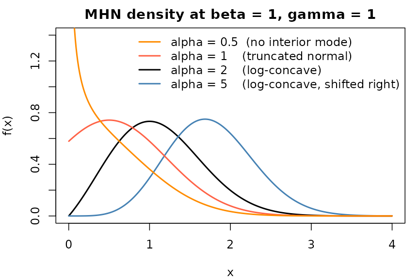

MHN density as alpha crosses the log-concavity threshold; beta = 1, gamma = 1 fixed.

The figure illustrates the qualitative claims developed in the next section. The density is log-concave whenever $\alpha \geq 1$ (Sun et al. 2023, Lemma 3a). For $\alpha > 1$ it has a finite interior mode in closed form (Sun et al. 2023, Lemma 3b); the borderline case $\alpha = 1$ reduces to the truncated normal, whose mode is $\max(0,\, \gamma/(2\beta))$ — interior when $\gamma > 0$, on the boundary $x = 0$ otherwise. For $\alpha < 1$ the density is typically monotone decreasing with a boundary singularity at $x \to 0^+$. The one exception is $\gamma > 0$ together with $\alpha \geq 1 - \gamma^2/(8\beta)$, where the density is not unimodal: it diverges at $x \to 0^+$, dips to a local minimum, rises to a single interior local maximum, and then decays (Sun et al. 2023, Lemma 3c). At $(\beta, \gamma) = (1, 1)$ this threshold is $1 - 1/8 = 0.875$, so the orange ($\alpha = 0.5$) curve in the figure sits in the strict monotone-decreasing regime, with no interior local maximum.

Shape and moments

Three facts from Sun et al. (2023) drive everything the package does with shape, moments, and the mode.

Log-concavity is a function of $\alpha$ alone (Sun et al. 2023, Lemma 3a). For $\alpha \geq 1$ the density is log-concave irrespective of $\beta$ and $\gamma$; for $\alpha < 1$ it is not. This single threshold is what splits the Gao & Wang (2025) RTDR sampler into its log-axis and original-axis branches in §6 below.

The mode has a closed form for $\alpha > 1$ (Sun et al. 2023, Lemma 3b):

$$X_{\mathrm{mode}} = \frac{\gamma + \sqrt{\gamma^2 + 8\beta(\alpha - 1)}}{4\beta}.$$

For $\alpha = 1$ the mode is $\max(0,\, \gamma/(2\beta))$ (the truncated-normal mode, Sun et al. 2023, Lemma 6b). For $\alpha < 1$ the density is either monotone decreasing or develops a non-trivial local maximum and local minimum, depending on the sign of $1 - \gamma^2/(8\beta) - \alpha$ (Sun et al. 2023, Lemma 3c–d). The helper mhn_mode() implements this case split and returns NA when no interior mode exists.

Moments satisfy a two-term recurrence (Sun et al. 2023, Lemma 2b):

$$E(X^{k+2}) = \frac{\alpha + k}{2 \beta}\, E(X^{k}) + \frac{\gamma}{2 \beta}\, E(X^{k+1}).$$

Together with the closed-form ratio for $E(X)$ in terms of $\Psi$ (Sun et al. 2023, Lemma 2a), this gives every higher moment. The helpers mhn_mean(), mhn_var(), mhn_skewness() and mhn_kurtosis() apply the recurrence in C++ via Rcpp; the Introduction vignette shows them in action. A useful sanity bound (Sun et al. 2023, Lemma 4c) is $\mathrm{Var}(X) \leq 1/(2\beta)$ for every $\alpha \geq 1$, $\gamma \in \mathbb{R}$.

The Fox–Wright $\Psi$ normalising constant

The normalising constant in the MHN density is

$$\Psi\!\left[\frac{\alpha}{2},\, z\right] \;=\; \sum_{n=0}^{\infty} \frac{\Gamma\!\big(\tfrac{\alpha + n}{2}\big)}{n!} \, z^{n}, \qquad z = \frac{\gamma}{\sqrt{\beta}}.$$

This series is absolutely convergent for every $\alpha > 0$ and every $z \in \mathbb{R}$, and is strictly positive. It depends on $(\alpha, \beta, \gamma)$ only through the two-dimensional combination $(\alpha, z)$.

A useful organisational point: $\Psi$ matters only for some of the package’s exported functions.

Function group	Needs $\Psi$?	Why
dmhn, pmhn, qmhn	yes	$\Psi$ sits in the density’s denominator and in the CDF series.
mhn_mean, mhn_var, mhn_skewness, mhn_kurtosis	yes	Moments are ratios $\Psi[(\alpha+k)/2,\, z] / \Psi[\alpha/2,\, z]$.
rmhn (Sun or RTDR path)	no	$\Psi$ enters both proposal scale and target as a common factor that cancels.

The practical consequence is that any numerical issues in evaluating $\Psi$ — accumulated rounding in lgamma, or truncation error in the series — can only affect d/p/q and the moment helpers; they cannot leak into the sampler.

For evaluation, the package follows the case split of Sun et al. (2023, Lemma 9–11):

• $\gamma = 0$ gives $\Psi[\alpha/2, 0] = \Gamma(\alpha/2)$.
• $\alpha = 1$, and the $\alpha = 2,\, \gamma \geq 0$ corner, both reduce to closed forms involving $\Phi$ (Sun et al. 2023, Lemma 9c).
• $\gamma > 0$ uses the alternating-free series of Sun et al. (2023, Lemma 10) with a pre-computed truncation point. All terms are positive, so there is no catastrophic cancellation.
• $\gamma < 0$ switches to the integral representation (Sun et al. 2023, Lemma 11) and uses Boost’s gauss_kronrod (for $\alpha \geq 1$) or tanh_sinh (for $\alpha < 1$, where the boundary singularity $u^{\alpha-1}$ needs the double-exponential rule).

Errata in Sun et al. (2023)

The published paper has two typesetting errors that touch the implementation. Each is corrected in the supplementary derivation, and the package follows the corrected form.

• Mixture weights $p_{i}$in Lemma 7. The main-text statement of Lemma 7 gives the weights for the $\sqrt{\mathrm{Gamma}}$ mixture representation as $p_{i} = \tfrac{1}{2\beta^{\alpha/2}} \cdot \tfrac{\Gamma((\alpha + 1 + i)/2)\, (\gamma/\sqrt{\beta})^{i}} {i!\, \Psi[\alpha/2,\, \gamma/\sqrt{\beta}]}$. These do not sum to one, contradicting the definition of $\Psi$ and the Poisson–Gamma hierarchical representation in Sun et al. (2023, Lemma 5a). The correct form, reproduced in the supplementary proof of Lemma 7 (Supplementary §2.13), is $$p_{i} \;=\; \frac{\Gamma((\alpha + i)/2)\, (\gamma/\sqrt{\beta})^{i}} {i!\, \Psi[\alpha/2,\, \gamma/\sqrt{\beta}]}$$ i.e. drop the leading $1/(2\beta^{\alpha/2})$ and use $\alpha + i$ in the $\Gamma$ argument instead of $\alpha + 1 + i$. This affects Algorithm 2 only, which the package does not implement; the correction is recorded here for completeness.

• Series truncation discriminants $C_{1}$, $C_{2}$in Lemma 10. The truncation point of the $\Psi$ series is the smallest $k$ for which $A(k+1)/A(k) \leq q$ (with an analogous bound for $B$). Reducing this to a quadratic in $k$ gives a discriminant whose last term is $\alpha x^{2}$ (and $(\alpha+1) x^{2}$ for $C_{2}$). The main-text statement of Lemma 10 prints these as $\alpha x$ and $(\alpha+1) x$ — a single missing power of $x$. The supplementary derivation (Supplementary §2.2.1, §2.2.2) carries $z^{2}$ throughout, in agreement with the rederivation. The corrected $x^{2}$ form is what the package uses in src/mhn_psi_series.cpp (marked with an // ERRATA comment); evaluating $\Psi$ at the published $x$ form would give a too-small truncation point and silently lose precision.

Sampling: Sun et al. (2023)

Sun et al. (2023) propose three Accept–Reject schemes, indexed by the sign of $\gamma$ and a coarse split on $\alpha$. Two of them — Algorithm 1 and Algorithm 3 — are implemented in the package and reachable via rmhn(method = "sun"). Algorithm 2 is not, and this section explains the reason.

Algorithm 1 — $\gamma > 0$, $\alpha \geq 1$

For each parameter triple, Algorithm 1 constructs two proposal distributions — a Normal with mean $\mu_{\mathrm{opt}}$ and variance $1/(2\beta)$, and a $\sqrt{\mathrm{Gamma}(\alpha/2,\, \delta_{\mathrm{opt}})}$ — each with a multiplicative envelope constant $K_{1}$ and $K_{2}$. Setup chooses whichever envelope is tighter ($K_{1} \leq K_{2}$ or the reverse). The two optima $\mu_{\mathrm{opt}}$ and $\delta_{\mathrm{opt}}$ have closed forms (Sun et al. 2023, Theorem 1b), so setup is cheap. The acceptance probability is bounded below by 0.8 for $\alpha \geq 4$ (Sun et al. 2023, Theorem 2e). For $1 \leq \alpha < 4$ no uniform lower bound is proved, but the original Figure 2 shows empirically high acceptance throughout that range.

Algorithm 3 — $\gamma \leq 0$

When the tilt is non-positive, Theorem 3 of Sun et al. (2023) supplies a proposal kernel based on an AM–GM-type inequality. With a tuning point $m > 0$ and the exponent $r = (\beta m + |\gamma|)/(2\beta m + |\gamma|)$, the candidate is

$$T \sim \mathrm{Gamma}\!\big(\alpha \cdot r,\, m(\beta m + |\gamma|)\big), \qquad X = m \cdot T^{r}.$$

The construction works for every $\alpha > 0$; the uniform acceptance bound $\geq 1/\sqrt{2} \approx 0.707$ (Sun et al. 2023, Theorem 4c) is proved only for $\alpha > 1$, but the procedure also samples correctly when $\alpha \leq 1$. The matching point is initialised from a closed-form heuristic of Sun et al. (2023, §4.2): $m_{\mathrm{init}} = \alpha^{2}/(1 + \alpha)$ for $\alpha \leq 1.1$ and a more elaborate expression based on the mode and the rightmost inflection point for $\alpha > 1.1$. The package then applies a single Newton-Raphson refinement step in both regimes, producing $m_{\mathrm{recommend}}$, whose acceptance probability is within $0.2\%$ of the optimum across the parameter range tabulated in Sun et al. (2023, Table 1).

Why Algorithm 2 is not implemented

Algorithm 2 targets $\gamma > 0$ with $\alpha < 1$ via the mixture representation

$$f_{\mathrm{MHN}}(x \mid \alpha, \beta, \gamma) \;=\; \sum_{i=0}^{\infty} p_{i}\, f_{i}(x \mid \alpha, \beta), \qquad f_{i} \;\sim\; \sqrt{\mathrm{Gamma}\!\big((\alpha + i)/2,\, \beta\big)}.$$

The mixture-component sampler needs a truncation point $M^{\dagger}$ chosen so that the tail mass beyond $M^{\dagger}$ is below a target tolerance (Sun et al. 2023, Lemma 8). For large $\gamma^{2}/\beta$ this truncation grows like $\gamma^{2}/(\varepsilon^{2} \beta)$, and the whole scheme degrades catastrophically — Gao & Wang (2025, Table 1) report a slowdown of up to $\sim 3 \times 10^{4}\times$ against RTDR in the most extreme case $(\alpha, \gamma) = (0.01, 10000)$. The package therefore declines to implement Algorithm 2 and routes $(\alpha < 1, \gamma > 0)$ to RTDR, where the acceptance bound $\geq 1/e$ (next section) holds uniformly.

Sampling: Gao & Wang (2025) RTDR

Gao & Wang (2025) introduce a Relaxed Transformed Density Rejection (RTDR) sampler that comes with a uniform lower bound on the acceptance probability across the entire parameter space. Three ideas drive the construction.

$T_{c}$-concavity

Standard TDR builds piecewise-linear envelopes on top of a log-transformed density. RTDR generalises to the $T_{c}$ family

$$T_{c}[x] = \mathrm{sign}(c) \cdot x^{c} \quad (c > -1,\, c \neq 0), \qquad T_{0}[x] = \log x.$$

A density $f$ is $T_{c}$-concave if $T_{c}[f]$ is concave. Logarithmic concavity (the usual TDR setting) is the $c = 0$ special case. The package’s RTDR implementation uses $c = -1/2$ on the log-axis density for the $\alpha < 1$ branches because $T_{-1/2}[x] = -x^{-1/2}$ accommodates the slower decay of $g(y)$ when the original $f$ has a boundary singularity at $x = 0$.

Working on the log axis when $\alpha < 1$

When $\alpha < 1$ the density $f(x \mid \alpha, \gamma)$ on $(0, \infty)$ blows up at the left endpoint and is not amenable to direct envelope construction. The change of variable $y = \log x$ yields

$$g(y \mid \alpha, \gamma) \;=\; \exp\!\big( \alpha y - e^{2y} + \gamma e^{y} \big), \qquad y \in \mathbb{R},$$

which is bounded and unimodal (Gao & Wang 2025, Lemma 3.3). RTDR operates on $g$ for $\alpha < 1$ and on $f$ directly for $\alpha \geq 1$.

The four regions

After scale normalisation $\sqrt{\beta} X \to X$ (so we may assume $\beta = 1$), the RTDR envelope construction splits into four regions based on $(\alpha, \gamma)$. The $\gamma$ in the table below is the normalised tilt $\gamma_{\mathrm{norm}} = \gamma/\sqrt{\beta}$; for a general $\beta$ the package’s rmhn(method = "rtdr") rescales internally and compares $\gamma_{\mathrm{norm}}$ against the boundary $2(1 - \sqrt{1 - 2\alpha})$.

Region	$\alpha$	$\gamma$	Envelope target	Reference
(a)	$\geq 1$	any	$f$ log-concave	Gao & Wang (2025, Theorem 3.1)
(b)	$[1/2,\, 1)$	any	$g$$T_{-1/2}$-concave	Gao & Wang (2025, Corollary 3.1; Theorem 3.2)
(c)	$(0,\, 1/2)$	$\leq 2(1 - \sqrt{1 - 2\alpha})$	$g$$T_{-1/2}$-concave	Gao & Wang (2025, Lemma 3.5; Theorem 3.2)
(d)	$(0,\, 1/2)$	$> 2(1 - \sqrt{1 - 2\alpha})$	$g$ with inflection at $y^{*} = \log(\gamma/4)$	Gao & Wang (2025, Theorem 4.4)

Region (a) is the easiest: $f$ is log-concave, two tangent lines and a constant segment suffice. Regions (b) and (c) reuse the same $T_{-1/2}$ envelope on $g$, with only the validity argument differing. Region (d) is the hardest — $g$ has an inflection point and the envelope needs $K$ secant segments on the log-convex side, with $K$ growing logarithmically in $\gamma$.

Why “relaxed”

The classical TDR construction asks for optimal tangent contact points, which generally have no closed form and must be found by Newton iteration. Gao & Wang (2025, Theorem 2.1) show that the acceptance bound $\leq e \approx 2.719$ (equivalently, acceptance probability $\geq 1/e \approx 0.368$) holds as long as the contact points lie anywhere inside a fixed interval — namely

$$\log\!\frac{f(m)}{f(t)} \in \begin{cases} [0.46,\, 2.49] & f \text{ log-concave (region (a))}, \\ [0.93,\, 1.99] & g \text{ $T_{-1/2}$-concave (regions (b), (c))}. \end{cases}$$

Setup is therefore a handful of cheap iterations that terminate as soon as the bracket is hit, with no need for a precise Newton solution. This is the main practical edge of RTDR over Algorithms 1 / 3 of Sun et al. (2023) in Gibbs-style workloads where $(\alpha, \beta, \gamma)$ changes every iteration: the setup cost is amortised over a single draw instead of many, and a cheap setup wins.

Composing the bounds in Gao & Wang (2025, Theorems 3.1, 3.2, 4.4) yields the headline guarantee of RTDR: for every $(\alpha, \beta, \gamma)$ with $\alpha > 0$, $\beta > 0$, $\gamma \in \mathbb{R}$, the acceptance probability is at least $1/e \approx 0.368$. The three algorithms of Sun et al. (2023) only have parameter-dependent guarantees (and only on parts of the parameter space — see §5).

A quick sanity check that the RTDR sampler converges to the right distribution in all four regions — empirical means from RTDR vs theoretical means across regions (a), (b), (c), (d), each based on 5000 draws:

cases <- data.frame(
  region = c("(a)", "(b)", "(c)", "(d)"),
  alpha  = c(2.0,    0.7,    0.3,    0.3),
  gamma  = c(0.5,    1.0,    0.5,    5.0)
)
set.seed(42)
empirical <- mapply(
  function(a, g) mean(rmhn(5000, alpha = a, beta = 1, gamma = g, method = "rtdr")),
  cases$alpha, cases$gamma
)
theoretical <- mapply(mhn_mean, cases$alpha, beta = 1, cases$gamma)
data.frame(cases,
           empirical_mean   = round(empirical,   4),
           theoretical_mean = round(theoretical, 4))
#>   region alpha gamma empirical_mean theoretical_mean
#> 1    (a)   2.0   0.5         1.0126           1.0016
#> 2    (b)   0.7   1.0         0.6442           0.6424
#> 3    (c)   0.3   0.5         0.2972           0.2823
#> 4    (d)   0.3   5.0         2.3321           2.3221

The four rows hit the right means to two-to-three decimal places — about the sampling tolerance at $n = 5000$.

The rmhn(method = "auto") dispatch

rmhn exposes three values of method: "sun" (force the Sun Algorithm 1 / 3 path), "rtdr" (force the Gao & Wang RTDR path), and "auto" (default). The "auto" route is the package’s recommendation; it composes the four shortcuts above into one decision tree (this is the Step 3.7.3 final form, confirmed by the benchmarks under inst/benchmarks/):

                  rmhn(n, alpha, beta, gamma, method = "auto")
                                    │
                                    ▼
       ┌─ alpha = 1, gamma = 0  →  half-normal       (Sun et al. 2023, Lemma 6c)
       │
       ├─ gamma = 0             →  sqrt-Gamma        (Sun et al. 2023, Lemma 6a)
       │
       ├─ alpha = 1             →  truncated normal  (Sun et al. 2023, Lemma 6b)
       │
       ├─ alpha < 1 and gamma > 0
       │      →  RTDR  (regions (b) / (c) / (d), Gao & Wang 2025, Theorems 3.2, 4.4)
       │
       ├─ alpha > 1 and gamma > 0
       │      →  Sun Algorithm 1                    (Sun et al. 2023, Theorems 1, 2)
       │
       └─ gamma < 0
              ├─ samples_per_setup ≥ 25  →  RTDR    (region (a))
              └─ samples_per_setup < 25  →  Sun Algorithm 3

Write $S$ for the samples_per_setup quantity in the last branch,

$$S \;=\; \max\!\Big(1,\; \frac{n}{\max(L_{\alpha},\, L_{\beta},\, L_{\gamma})}\Big),$$

where $L_{\alpha}$, $L_{\beta}$, $L_{\gamma}$ are the recycled lengths of the three parameter vectors. The intuition follows from decomposing the expected time per draw as

$$E[\text{time}/\text{draw}] \;=\; \frac{T_{\text{setup}}}{n} \;+\; C_{\text{reject}} \times T_{\text{per-proposal}},$$

where $T_{\text{setup}}$ is the one-off cost of preparing the proposal (a single $m_{\text{init}}$ formula plus at most one Newton step for Sun Algorithm 3; an iterative contact-point search for RTDR), $C_{\text{reject}} = 1/\text{acceptance}$ is the expected number of proposals per accepted draw, and $T_{\text{per-proposal}}$ is the cost of one proposal cycle (sample plus acceptance log-ratio evaluation).

For $\gamma < 0$ the two samplers sit on opposite ends of this trade-off:

• Sun Algorithm 3 has a cheap setup — $m_{\text{init}}$ has a closed form, and the optional Newton refinement uses one boost::math::digamma evaluation — but a more expensive per-proposal: every proposal calls rgamma, evaluates the fractional power $X = m \cdot T^{r}$, and the acceptance log-ratio carries the same $(X/m)^{1/r}$ term.
• RTDR (region (a)) has a more expensive setup: each contact point $t_{l}$, $t_{r}$ is found by an iterative search that terminates as soon as $\log f(m)/f(t)$ lands in the bracket $[0.46,\, 2.49]$. But the per-proposal is light: sampling from the piecewise envelope is straight arithmetic plus a single log, and the acceptance ratio adds only two more logs.

When $S$ is large the per-proposal term dominates and RTDR wins; when it is small — the Gibbs case where each iteration redraws $(\alpha, \beta, \gamma)$ — the setup term dominates and Sun Algorithm 3 wins. The crossover at 25 is the round value chosen inside the empirical break-even window $n \in [10,\, 25]$ observed at every one of the 20 surveyed $(\alpha, \gamma)$ cells in inst/benchmarks/auto_dispatch.R.

A small concrete demonstration: with set.seed aligned, method = "auto" and the expected forced method produce bit-identical draws on each branch.

# Branch: alpha < 1 and gamma > 0  -->  expects RTDR
set.seed(7); auto1 <- rmhn(20, alpha = 0.7, beta = 1, gamma = 2)
set.seed(7); rtdr1 <- rmhn(20, alpha = 0.7, beta = 1, gamma = 2, method = "rtdr")
identical(auto1, rtdr1)
#> [1] TRUE

# Branch: alpha > 1 and gamma > 0  -->  expects Sun Algorithm 1
set.seed(7); auto2 <- rmhn(20, alpha = 3,   beta = 1, gamma = 2)
set.seed(7); sun2  <- rmhn(20, alpha = 3,   beta = 1, gamma = 2, method = "sun")
identical(auto2, sun2)
#> [1] TRUE

# Branch: gamma < 0 with samples_per_setup < 25  -->  expects Sun Algorithm 3
set.seed(7); auto3 <- rmhn(5,  alpha = 2,   beta = 1, gamma = -1)
set.seed(7); sun3  <- rmhn(5,  alpha = 2,   beta = 1, gamma = -1, method = "sun")
identical(auto3, sun3)
#> [1] TRUE

The three TRUE outputs are the same invariant that tests/testthat/test-rmhn.R enforces as a regression test.

References

Sun, J., Kong, M., & Pal, S. (2023). The Modified-Half-Normal distribution: Properties and an efficient sampling scheme. Communications in Statistics – Theory and Methods, 52(5), 1507–1536.

Gao, F. & Wang, H.-B. (2025). Generating modified-half-normal random variates by a relaxed transformed density rejection method. Communications in Statistics – Simulation and Computation.

Robert, C. P. (1995). Simulation of truncated normal variables. Statistics and Computing, 5(2), 121–125.